Data Cleaning in Excel Best Practices & Tips

Using Excel is great for managing, organising, and analysing your data. However, some datasets are full of inaccurate and inconsistent data, which is often called dirty data. To fix this data and ensure you can actually use it to gain important insights, you need to clean it.

Data cleaning in Excel is all about correcting errors and other issues in your data so it's usable for reporting and analysis.

This guide goes over why data cleaning is so important, some common pitfalls to avoid, and some of the best data cleaning techniques to use.

For advice on other hot topics, explore our full list of Excel courses!

Why Data Cleaning is Essential in Excel

There are several reasons why data cleaning in Excel is so important. It helps you to:

• Fix inaccuracies in your data, like extra spaces, spelling errors, or missing values
• Boost data consistency by standardising formats and values
• Improve your business decision-making, as you have accurate data to base decisions on
• Increase worker productivity and efficiency, as they don’t need to waste time manually tracking down data

Common Data Issues in Excel

When dealing with dirty datasets in Excel, there are several common issues you’ll likely run into. This includes:

• Inaccurate data (such as wrong numbers, spelling errors, or incorrect calculations)
• Inconsistencies (such as different formats or different names for the same person or item)
• Duplicate data
• Raw or unstructured data
• Incomplete data, or data that’s missing altogether
• Hidden data
• Stale or outdated data

Dealing with all or any of these issues can make analysing and making sense of your data very challenging and time-consuming.

Key Techniques for Data Cleaning in Excel

Thankfully, there are several simple techniques you can use in Excel to combat and fix some of these common data issues.

Removing Duplicates

It’s incredibly simple to remove duplicates from your dataset columns in Excel.

1. Go to the Data tab, and click Remove Duplicates.

2. In the window that pops up, select the column that you’d like to remove duplicates from.

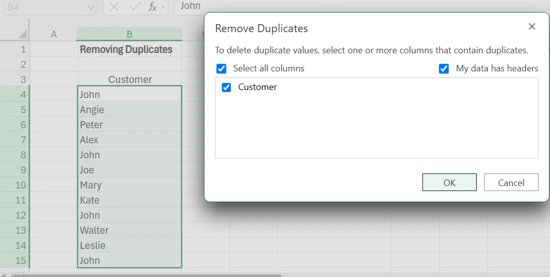
3. After clicking okay, another pop-up will appear that tells you how many duplicate values were found, and how many unique values remain in the column. It’ll also automatically remove the duplicates from the dataset.

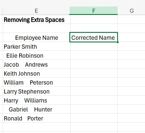
Removing Extra Spaces

Extra spaces before, after, or during text strings can introduce formatting and analysis problems, and are notoriously difficult to spot manually. To remove these extra spaces, use the TRIM function in Excel. In this example, we’re going to highlight how this function can remove the extra spaces in an employee name database.

1. Next to your column of data that you want to remove extra spaces from (in this case, our employee name list), add another helper column called “Corrected Name”.

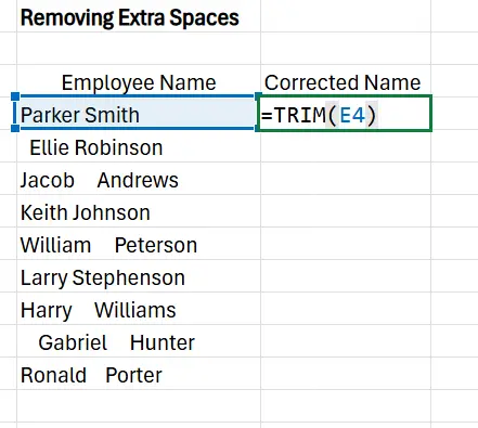
2. In the first cell of the new column, enter =TRIM(cell with the text). So for our example, it’ll be E4, as that’s the cell that contains Parker Smith.

3. Drag the formula down by clicking the bottom right corner of the first cell in the “Corrected Name” column, and dragging it throughout the rest of the cells in the column. You’ll see this “Corrected Names” column populate the correct names without the extra spaces.

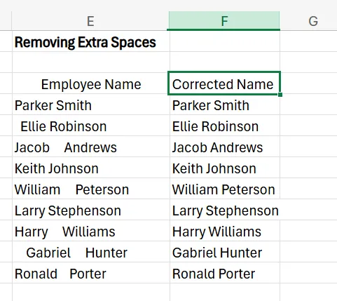
4. Lastly, simply copy the results from the “Corrected Name” column and paste them back in the original column. Once everything is moved over correctly, you can delete the helper column.

Fixing Character Cases

If you require text to be in a certain character case within your dataset (such as lower case, upper case, sentence case, etc), trying to fix this issue manually is a painstaking process that may take hours. Instead, you can just use the PROPER, UPPER, or LOWER function.

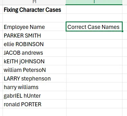
In this example, let’s say a company requires that its employee database be in a format where the first letter of both the first and last name is capitalised, while the other letters are lowercase.

1. Next to your employee list that’s full of improper capitalisation, create a helper column, which in this case we’ll call “Correct Case Names”.

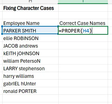
2. In the first cell of the new column, enter =PROPER(cell with the text). In our example, this will be =PROPER(H4), as H4 is the cell where the first person’s name is.

3. Drag the formula down across the rest of the column to apply it to every name.

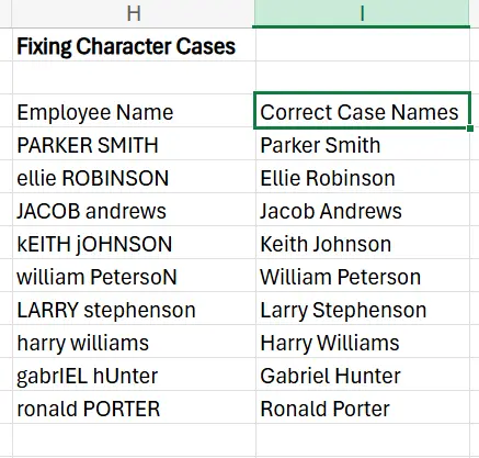
4. You can copy the names from the new column, paste them into the old column, and then delete the helper column.

5. If you want to use the UPPER or LOWER function instead, simply substitute =UPPER or =LOWER instead of =PROPER in the syntax we mentioned above.

Standardising Values

To ensure that all values, words, and terms are standard throughout the dataset, you can use the convenient Find and Replace feature. This lets you find a certain term or value, and replace it with something else. In our example, we want to standardise the way that the United States is referred to in its customer database.

You’ll see that some of the data has it correct (United States), while others refer to it as the United States of America.

1. In your dataset, click Ctrl + H to open the Find and Replace feature.

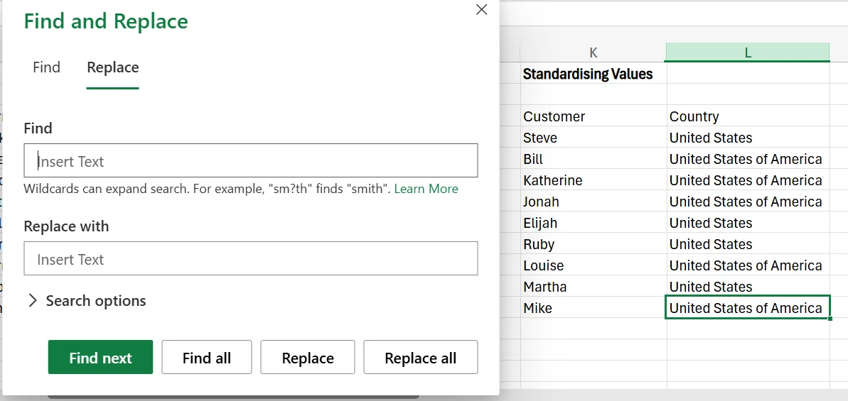
2. Next, put “United States of America” in the Find box, and then the standardised value of “United States” in the Replace With box.

3. After clicking Replace all, it’ll automatically replace the matches, and even tell you how many terms were replaced.

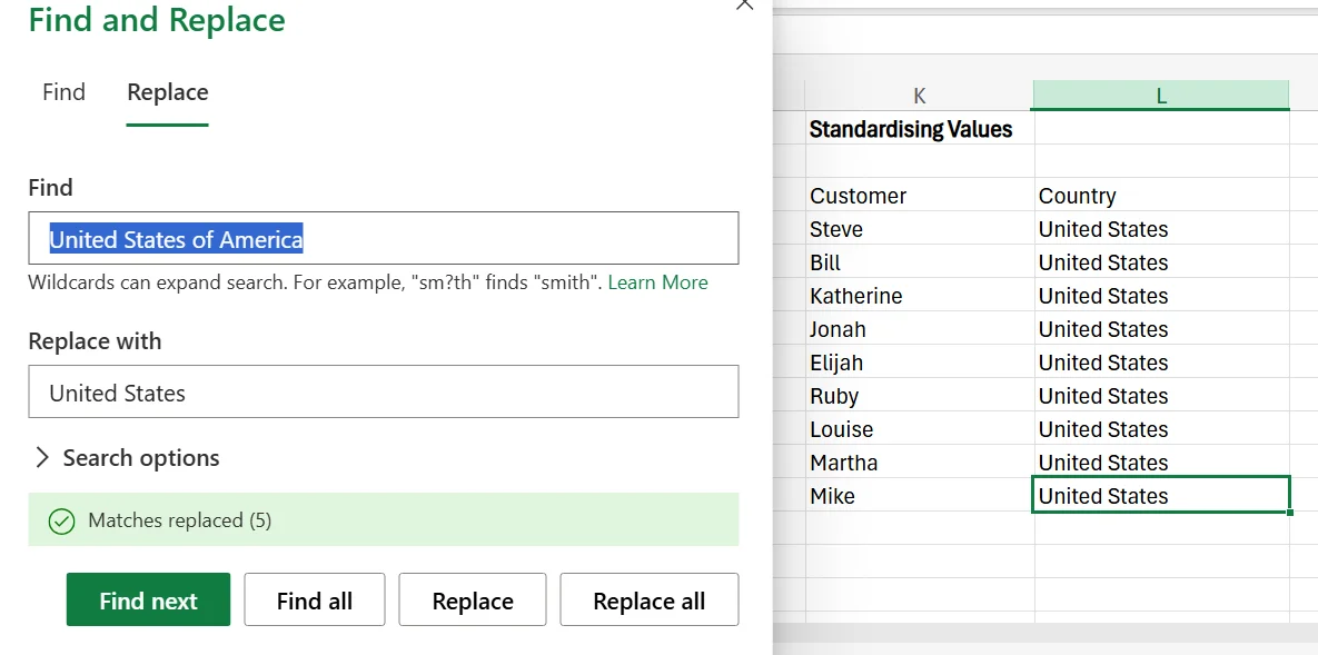
4. This feature only lets you do one value at a time, so if you have another incorrect value in the dataset (such as USA or US), you’ll have to repeat these steps for each one.

Best Practices for Data Cleaning in Excel

While choosing the right techniques for data cleaning is important, there are also some best practices to be aware of.

Have Clear Guidelines

First, you need to establish clear guidelines about how data should be cleaned and what “clean data” actually means in your case. If it’s not clear what your standards or expectations are for clean data, some people may have different assumptions, which leads to even more inconsistencies in your datasets going forward.

Train Your Staff Well

In addition to guidelines, it's a good idea to take time to train your staff well on the various methods you need them to use to clean data. While most are straightforward, this training ensures they know what to do, and are aware of the features you want them to use.

Even one person doing things incorrectly or missing steps can ruin the consistency and usability of your data, so make sure everyone is confident and knowledgeable about what you need them to do. This training also helps team members feel more confident in their abilities, and helps your team buy into the value of data cleaning while also boosting accountability.

Monitor Your Data Quality

Monitoring your data quality can be great for making sure your current guidelines are suitable, or if more changes are needed to achieve results that you’re happy with. It also helps you catch small issues in your data before they become major concerns.

Troubleshooting and Common Pitfalls in Data Cleaning

While data cleaning is a great way to boost the accuracy, usability, and quality of your datasets, there are also some pitfalls and mistakes that companies make when cleaning data.

Overcleaning

Overcleaning your data involves going too far in your data cleaning efforts, where you end up accidentally changing or removing things that never should have been adjusted. Overcleaning may lead to skewed results, losing valuable data, altered formats, and may generally hurt your data quality more than it helps.

To avoid this, always ensure you have justification for why certain data needs to be cleaned, and be specific about what should be cleaned and what gets left alone.

Not Saving Backups

Before you attempt to clean data, it’s valuable to save a backup. You should also be saving backups throughout the cleaning process. Accidents happen, and if you accidentally delete or change important values while cleaning, having a backup ensures you don’t lose this valuable information.

Not Dealing With the Source of the Issue

While cleaning data is great, it doesn’t address the source of the issue in the first place. If you never address the root cause of the error, you’ll likely continue to see dirty data that suffers from similar errors in the future.

Instead of just cleaning the data, consider investigating why it’s inaccurate or inconsistent in the first place, and see if there’s a way to prevent it from happening going forward.

At Future Savvy we offer instructor-led training programs suitable for both beginners and advanced users. If you want to learn more about how we can help you and your team grow your business, contact us today!