How to Use Excel Lookup with Multiple Criteria

The LOOKUP functions in Excel let you easily find a value within a table and retrieve a corresponding value from a different row or column. You can also use these functions to find values based on multiple conditions or criteria.

This lets you find an employee's salary by searching their employee ID and job title, or lets you look up a customer’s name and a product to see how much of that item they’ve purchased from you. Being able to quickly and accurately retrieve data like this saves you plenty of time and effort while working with complex or comprehensive spreadsheets.

This guide looks closely at how to use Excel LOOKUP functions with multiple criteria, as well as goes over the potential business applications that these functions have. Explore our list of Excel courses for tips and advice on other topics!

How to Use Excel Lookup with Multiple Criteria

The concept behind using Excel LOOKUP with multiple criteria is to use formulas and combined values to be able to locate the exact column and row where the specific data you’re looking for resides.

To illustrate this process, we’re going to go through a step-by-step example. In this example, imagine that you’re a company that wants to see the sales data for different employees in a specific region.

Using XLOOKUP With Multiple Criteria

We’ll begin by going through a step-by-step example using the XLOOKUP function.

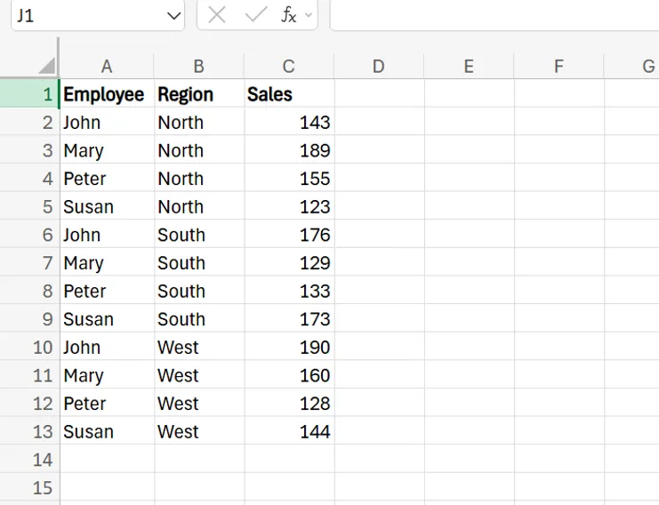
1. Begin by opening and/or setting up the spreadsheet that features your employee names, the regions you sell products in, and the sales numbers of the employees in each region.

2. Next, you need to define your criteria. In this case, let’s say we're looking for the amount of sales that Susan had in the South region. As a result, our criteria would be Susan and South.

3. Next, we’ll use the XLOOKUP function to find the sales value based on our criteria. The syntax for the XLOOKUP function is =XLOOKUP(lookup_value, lookup_array, return_array, [if_not_found], [match_mode], [search_mode]).

In this function, the lookup value is the values we are looking up (in this case, the name Susan and the region South), the lookup array is the range of each of those columns, and the return array is the data we want to get back, which in our example is the sales numbers. The rest of the syntax says what Excel should display if no match is found, the type of match you want, and how the function should search your data.

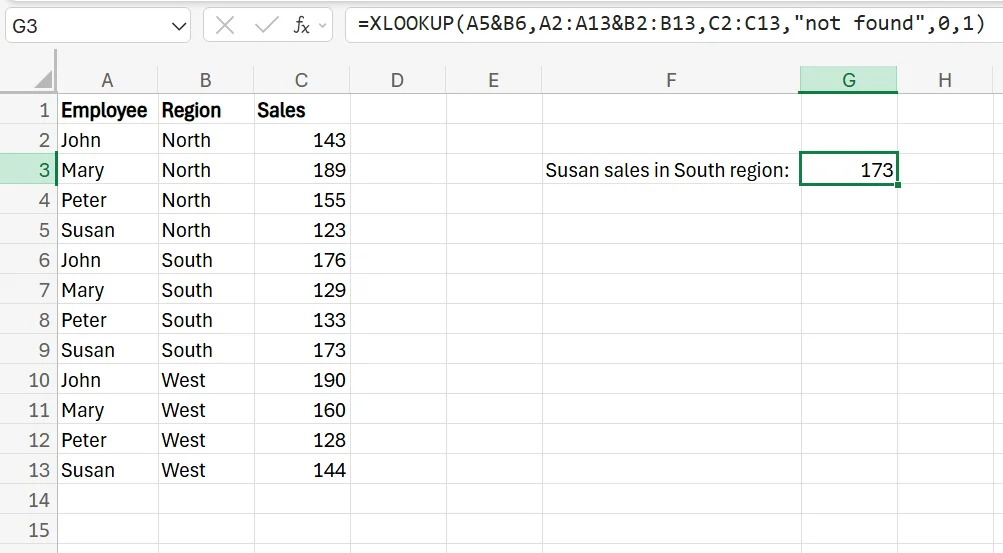
For our example, using the above data, the syntax for this function is =XLOOKUP(A5&B6,A2:A13&B2:B13,C2:C13,"not found",0,1). This function works, as you can see it correctly determines that Susan’s sales numbers in the South region were 173.

Here’s how we arrived at that syntax. After adding =XLOOKUP and an open bracket, we’ll click on the name Susan (we chose cell A5), add an ampersand, and then click on the South region (we chose cell B6).

Next, add a comma, and then select the range for the employee column (A2 to A13), add another ampersand, and then select the range for the region column (B2 to B13), after another comma, select the range for the Sales column (C2 to C13).

After that, add another comma and choose the text you want to appear if no results are found, and add it between two apostrophes. Type another comma and then choose the match type (we chose 0 for exact match only, and then add another comma and then choose the search mode to use (we chose 1, so it searches from the first result to the last). Then, finish up by closing the bracket and hitting Enter.

If you want to confirm it’s working, you can repeat the process and syntax with another name and region to see if it works.

While the Excel LOOKUP function with multiple criteria may not be needed in a dataset as small as our example, if you had hundreds of employees and numerous regions and sub-regions, this function would have a lot more value and save you lots of time when searching for sales data.

Using VLOOKUP and Helper Columns As an Alternative

Another option is to use the VLOOKUP function. While it’s not quite as easy as you need to create a helper column (as VLOOKUP only works with a single lookup value), it’s still an effective method.

1. Begin with the same dataset full of your employee names, regions, and sales numbers.

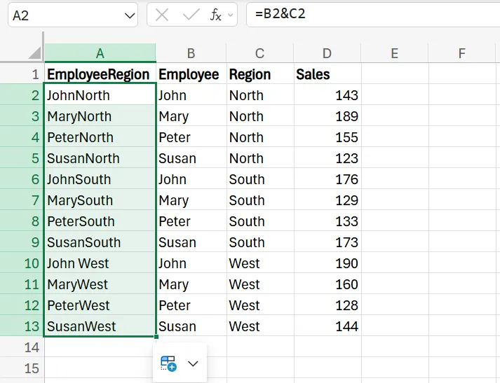
2. Create a helper column in the dataset. In our example, we’ll add an “EmployeeRegion” column. To populate the column, enter the formula =B2&C2 in the first cell, and click Enter. In the bottom right corner of the first cell in the column, click and drag the formula down to add it to the rest of the cells.

3. Now, you’re able to use the VLOOKUP FUNCTION to find Susan’s sales in the South. The syntax for this function is =VLOOKUP(lookup_value, table_array, col_index_num, [range_lookup]). You’ll add this function/formula to a cell you create off to the side.

Inside this formula, the lookup value is the value you’re searching for, the table array is the entire table, the col index num is the number of the column you want the return value to be from, and the range lookup is either True (for approximate match) or False (for exact match).

In our example, the function will look like this: =VLOOKUP(B5&C6,A2:D13,4,FALSE).

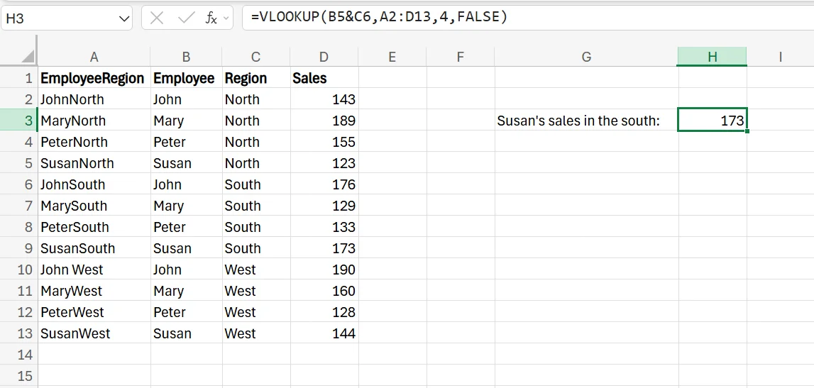
To get to this syntax, we add =VLOOKUP and an open bracket to our designated cell where we want Susan’s sales in the south to appear. Next, click the name Susan, add an ampersand, and then click South.

Add a comma and then drag your mouse over the entire table, add another comma, and then add a 4. This is because the Sales appear in the fourth column of our table. Finally, finish it off with another comma, False (as we want the exact value), close the bracket, and then click Enter.

As you can see, we arrive at 173 sales, which is the same result as the XLOOKUP function.

In addition to these two choices, you can also use the INDEX MATCH and FILTER functions for more advanced scenarios.

Potential Business Applications For Using Excel Lookup With Multiple Criteria

There are many ways that businesses can use these Excel LOOKUP functions to streamline and optimise their operations. First, it helps you analyse sales data by matching multiple conditions to ensure you only get the data you’re looking for, and aren’t overwhelmed with unrelated information.

For example, let’s say you want to find out how much of a certain product an employee sold in a particular region. Using one of these functions not only stops you from having to search manually, but also prevents you from being bombarded with additional data and details you’re not looking for. They’re efficient functions that only provide you with the exact information you want.

This saves you plenty of time and effort, and the functions give you plenty of flexibility to look up any combination of data that you need, no matter how precise it may be.

These LOOKUP functions can also have a variety of other business uses, such as checking calculations, tracking your stock and inventory levels, looking up employee information, updating compensation, forecasting sales, boosting the accuracy of your reports, and more.

To discover more detailed use cases and advanced business techniques, don’t hesitate to contact us!