- TIPS & TRICKS/
- How to Password Protect Excel & Hide a Single Column/


How to Password Protect Excel & Hide a Single Column
- TIPS & TRICKS/
- How to Password Protect Excel & Hide a Single Column/
How to Password Protect Excel & Hide a Single Column
How to Password Protect Excel and Hide Just One Column in a Master Spreadsheet
You can never be too careful when working with several people on a spreadsheet. You may need to hide sensitive data and lock the document.
Follow our step-by-step guide to hide columns and password-protect an Excel worksheet.
Are you wondering about the right type of training that your teams needs, but are unsure where to start?
Download our Training Needs Analysis Form
 Download now
Unlock All Cells
Unlocking all the cells in the sheet ensures that only the specific columns or cells you select are locked when you protect the sheet.
Tip: By default, all the cells in Excel are locked but this only takes effect when you protect the sheet.
1. Navigate to the Select All button and select it. The button is found at the top-left corner of the sheet where the row numbers and column letters intersect.
2. Right-click any cell or area in the sheet.
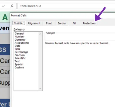
3. Select Format Cells from the menu.
4. In the dialog box, select Protection
5. Uncheck Locked and select OK.
Lock the Columns You Want to Protect
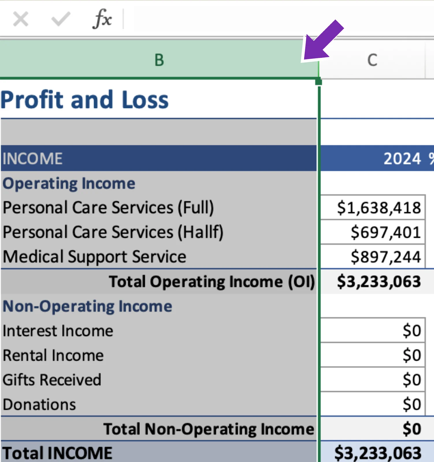
Columns are represented by letters while numbers represent rows.
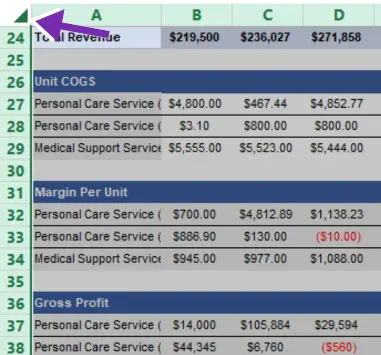
1. Select the letter that represents the column you want to lock.
2. Right-click the selected column.
3. Select Format Cells from the menu.
4. Select Protection in the dialog box.
5. Check the Locked option and select OK.
6. To hide the locked column, right-click anywhere on the selected column and choose Hide.
Protect the Sheet
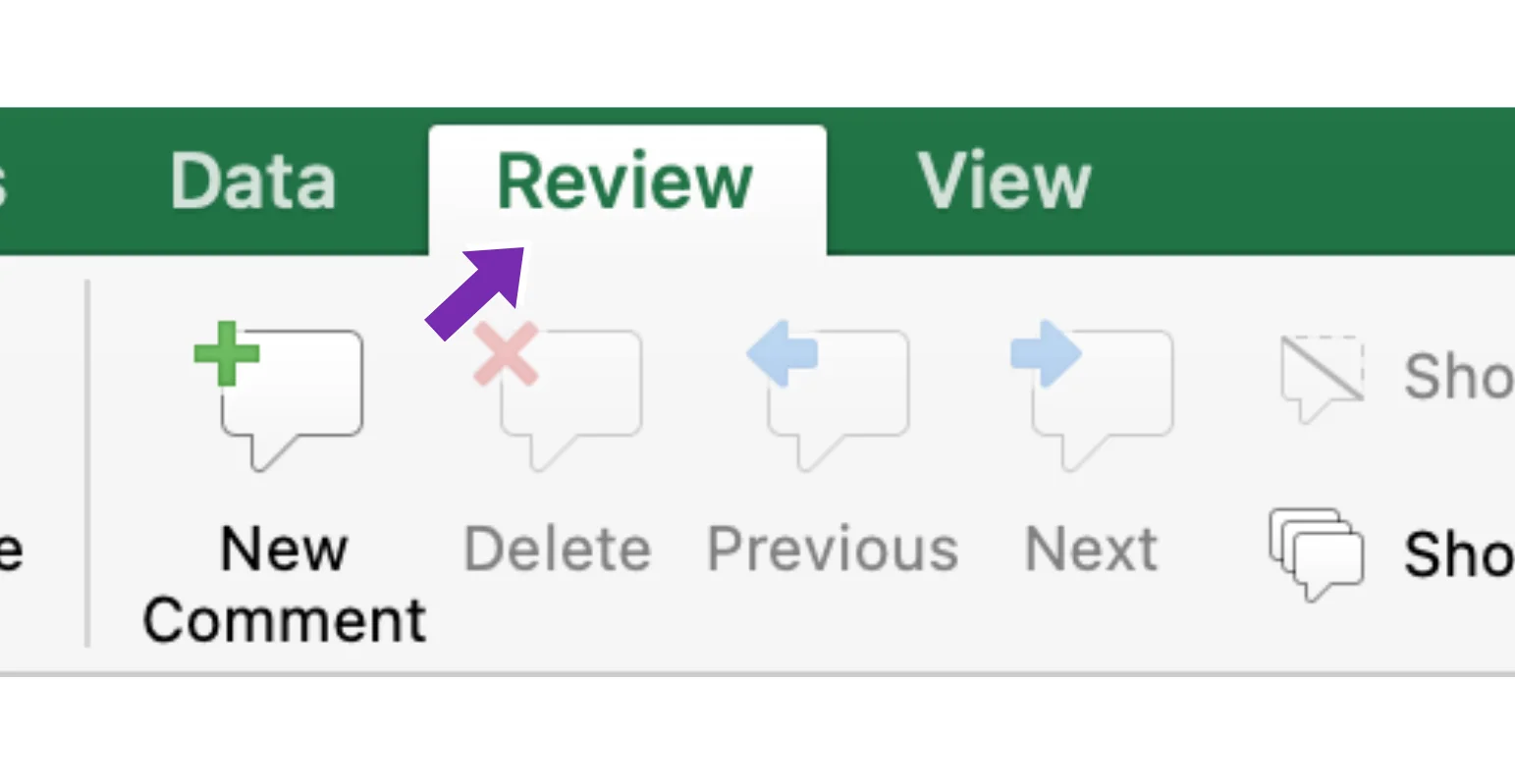
1. Navigate to the Review tab on the Ribbon and select it. The Ribbon, also known as the toolbar, is at the top of the Excel window. The ribbon houses several tabs, including File, Home, Review, Data, and Formulas.
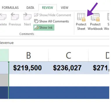
2. Select Protect Sheet.
3. In the dialog box, enter a password to password-protect your worksheet. You can also set user permission or role by checking and unchecking necessary boxes.
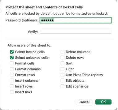
4. Re-enter your password and select OK.
You can still access the rest of the unlocked rows and columns but must provide a password to access the locked columns.
Download our Excel Skills Self-Assessment Questionnaire
 Download now
Can People Still Access Excel Worksheet after Protecting It with a Password?
Protecting your worksheet with a password should block unauthorised access. However, even without a password, some people may use third-party apps to gain entry. Use the Backstage View in the File tab for advanced security.
Related Articles
 Tips & Tricks
Can you Calculate Variance Using Excel?
In this guide, we explain variance as a measure of how widely data points deviate from the mean and shows why understanding this spread is useful for deeper insight and risk assessment. It walks readers through calculating variance in Excel, distinguishing between the VAR.S function for a sample and VAR.P for an entire population, then demonstrates each with a car-sales case study.
 Tips & Tricks
How to Use Excel Lookup with Multiple Criteria
This blog explains how Excel’s LOOKUP functions—particularly XLOOKUP and VLOOKUP—can retrieve data based on multiple criteria. It walks through a step-by-step example of finding an employee’s sales in a specific region, showing both an XLOOKUP formula and a VLOOKUP alternative that uses a helper column.
- Tips & Tricks
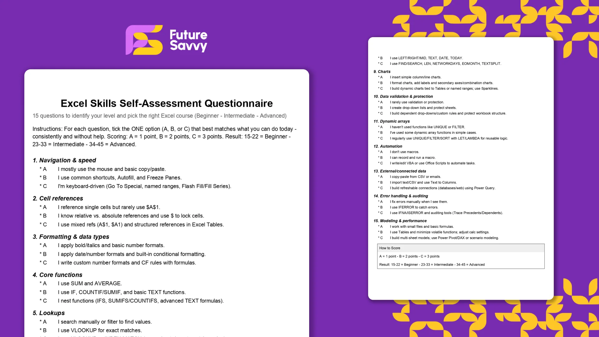
Excel Skills Self-Assessment Questionnaire
This free, printable Excel Skills Self-Assessment helps you quickly gauge your level and pick the right next step in your learning path. It contains 15 multiple-choice questions spanning navigation, formulas, lookups, tables, PivotTables, charts, dynamic arrays, Power Query, and more. You’ll score yourself and interpret the result to see whether you’re Beginner, Intermediate, or Advanced - then follow tailored course recommendations based on your score.