How to Aggregate Data in Excel

Excel is an incredibly popular tool for managing, storing, and analysing data. However, if your dataset is full of errors, hidden rows, or missing data, making accurate calculations may prove challenging.

Thankfully, you can use the AGGREGATE function to help overcome these issues and successfully make calculations to simplify or refine your data. Not only is it a useful function, but it’s also relatively easy to perform.

This guide takes you through the steps of using this function in Excel, the business use cases for it, and more.

How to Aggregate Data in Excel

To aggregate data in Excel, you need to use the AGGREGATE function. It’s a function that lets you perform calculations on your data, with the added flexibility of handling common issues like missing data, hidden rows, or errors.

The syntax for using this function is =AGGREGATE(function_num,options,range). The “function_num” refers to the number value of the exact function you want to use, such as Average, Count, Max, or Min. The “options” refer to which values you want to ignore in your calculation, while “range” refers to the actual cells you want to include in the aggregate.

Instructions for Aggregating Data in Excel

Now that you know what the function for aggregate in Excel is, let’s have a look at how to use it in practice.

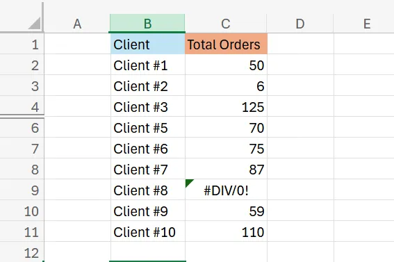
For this guide, we're using an example of a company that wants to calculate its total orders, the number of clients that made orders, and the average orders per client. Here’s a snapshot of its data.

As you can see from the data, not only is there a client missing from the dataset (Client #4 is hidden), but there’s also an error for the total orders of Client #8. If you try to do a simple SUM, AVERAGE, or COUNT function, you’ll get an error as a result. That’s where the AGGREGATE function comes in handy.

To use the aggregate function to calculate the total orders, create an “Aggregate total orders” cell, and add the following syntax: =AGGREGATE(9,3,range).

The “9” is for the “SUM” function, and the “3” means that the calculation ignores hidden rows and error values. For the range, you’ll simply drag and select all of the cells and press Enter to complete the calculation.

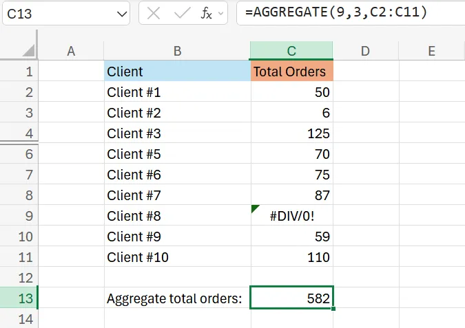
As you can see, this calculation tells us that there were 582 total orders.

On the other hand, if you want to use it to calculate the number of clients that made orders, create an “Aggregate total clients with orders” cell, and include the syntax: =AGGREGATE(2,3,range).

The “2” refers to the “COUNT” function, while the “3” and “range” are the same as the last calculation.

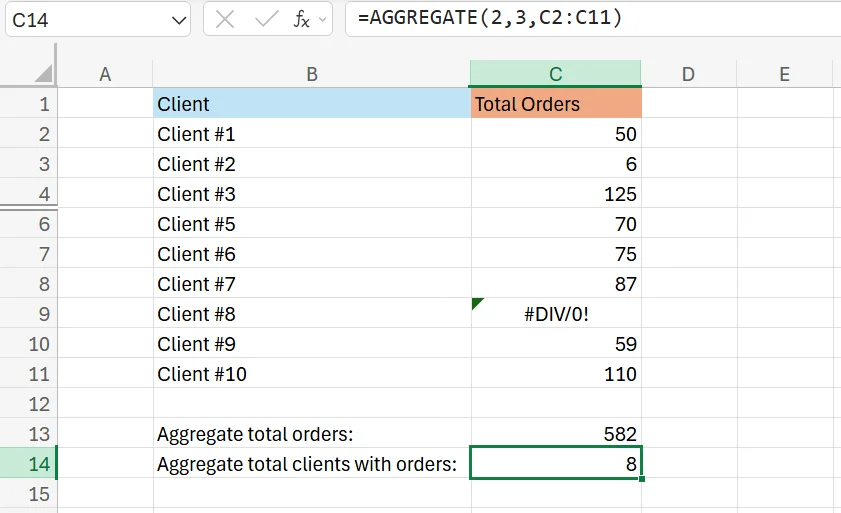
The calculation shows us that 8 clients in total have made orders.

Finally, to use it to calculate the average orders per client, create an “Aggregate average orders” cell and add the syntax: =AGGREGATE(1,3,range). The “1” refers to the “AVERAGE” function, while the other values are the same as the previous calculations.

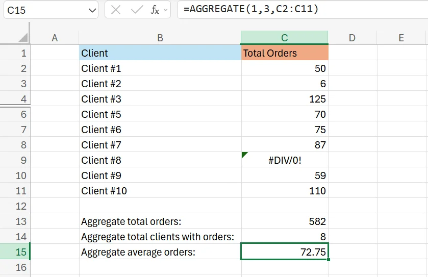
The calculation shows that the average client makes 72.75 orders.

While this example is fairly basic and simple, as there are only a handful of clients and data, the same practices and techniques can be used on much larger and more complex datasets.

To learn more about aggregating data in Excel, be sure to explore our dedicated article on advanced Excel aggregation techniques and business analytics (link).

Potential Business Applications for Aggregate in Excel

There are several reasons businesses can benefit from using the AGGREGATE function in Excel. Organisations may use it to streamline reports, simplify complex datasets, or generate dynamic summaries.

The function is also great for improving data quality by filtering out errors and missing data, to ensure that calculations are as accurate as possible. It also helps companies analyse sales and revenue, manage inventory (and calculate its value), and even examine data from marketing campaigns.

Aggregating data is also useful for internal HR tasks like calculating the average salary of your team, the number of total employees you have, or measuring the individual performance of different staff members.

Future Savy’s instructor-led training programs can help you gain valuable insights on your business. Get in touch today!