How to Remove Table Format in Excel

Using tables in Excel is often useful for better data management or analysis, and there are several different ways to format and customise them to your liking. While this formatting can help them look better and be easier to understand, there may be times when you want to rid the table of any formatting and take it back to square one.

Thankfully, the process for doing this is incredibly simple, and you won’t need to worry about losing or ruining your valuable data. This guide is going to show you how you can go about removing table format in Excel in only a few short steps.

Want to learn more about Excel’s features? Our instructor-led Excel training courses are suited for both beginners and advanced users.

What Is Excel Table Formatting?

Table formatting in Excel is the process of adding different styles of custom formats to a table or range of cells. This table formatting often has the goal of making your data more visually appealing and easier to organise and analyse.

The formatting could be adding colourful borders, different fonts, unique headers, filters, highlighting cells based on their content, and more.

Reasons to Remove Table Format in Excel

Despite table formatting working well in many situations, there are some reasons why you may want to remove all the formatting from your table.

Maybe the table was incorrect or had an issue, or you simply prefer to have the data laid out plainly. Also, removing the table format may help with compatibility issues and may decrease file size, which is especially useful if your dataset is very large. Some functions of Excel may not work as seamlessly with a table as they do with a range, as well.

How to Remove Table Format: A Step-by-Step Guide

The process to remove the formatting from your table in Excel is incredibly straightforward.

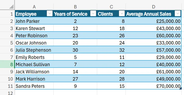
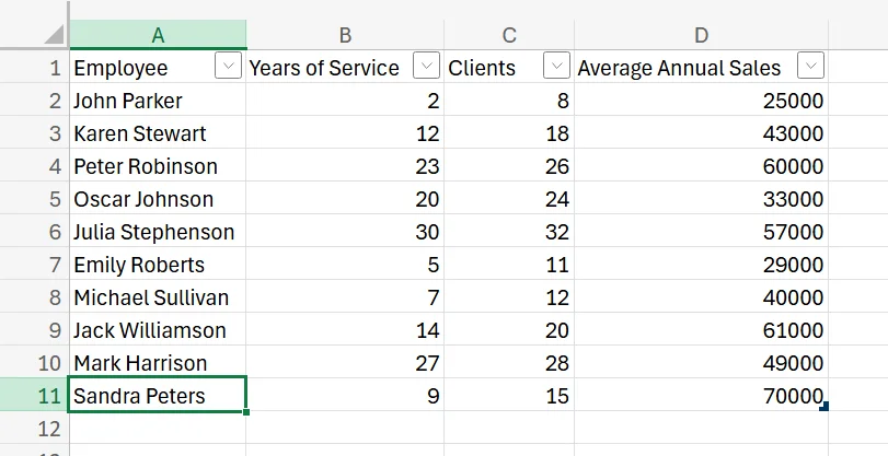
1. Open your dataset that includes your table in Excel. For this example, our table is a record of employees at a company, and it includes their name, their years of service, how many clients they have, and their average annual sales.

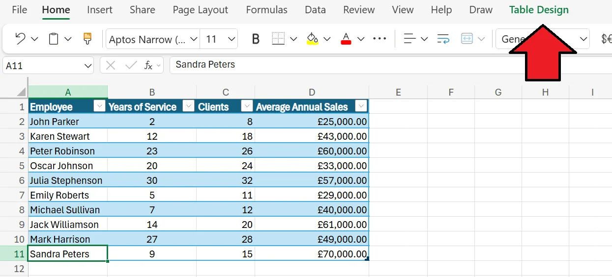
2. After clicking on one of the cells in your table, navigate to the Excel ribbon and click Table Design.

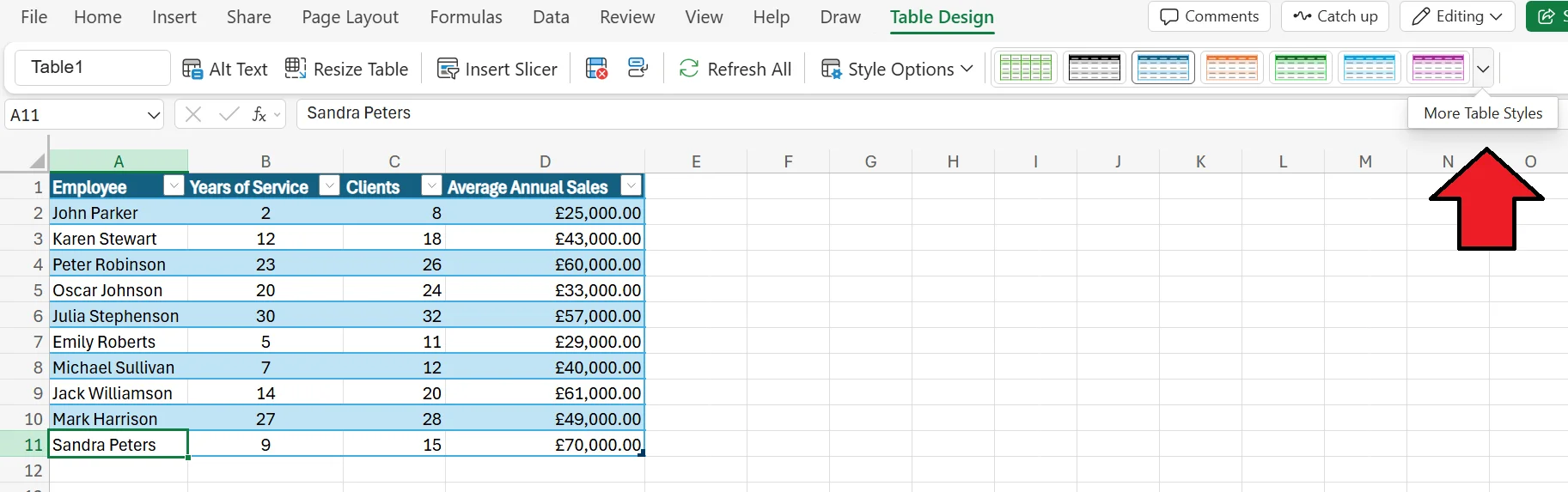
3. After clicking on Table Design, click the downward arrow next to the table styles to open up More Table Styles.

4. In the More Table Styles menu, choose None from the list of options.

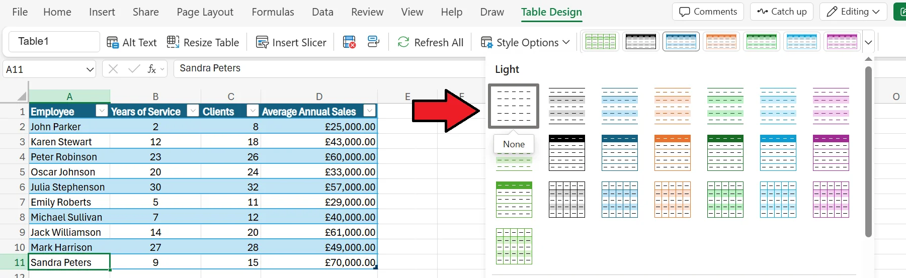
5. After clicking None, all the formatting will be automatically removed from your table.

Converting a Table to a Range in Excel

In addition to removing the formatting from a table, you can also convert the table to a range if you want to completely get rid of it.

1. Open your dataset that features your table, just like with the last example.

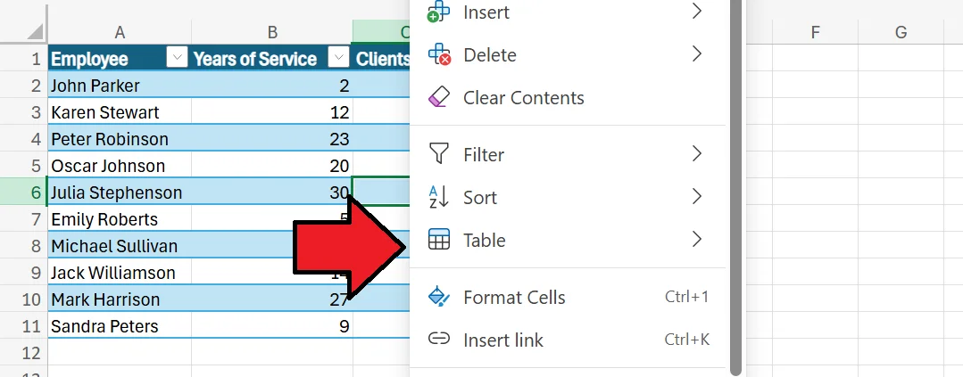
2. Next, right-click anywhere on your table and then from the dropdown menu, hover over Table.

3. From the list of options that pops up, click Convert to Range.

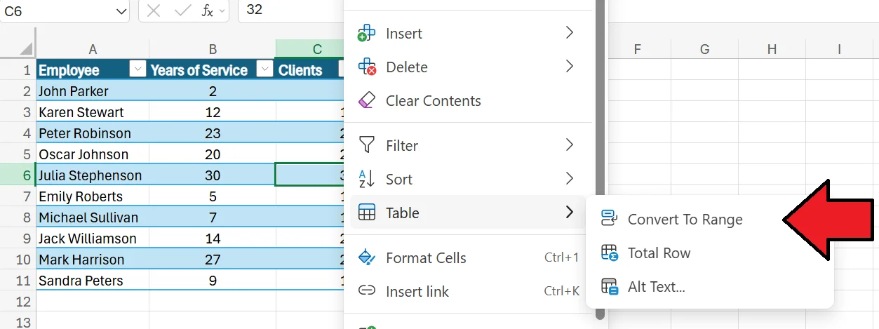
4. Once you click Convert to Range, your table is automatically transformed into a range of cells, as opposed to a table.

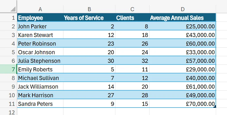
5. If you want to remove all the colours/shading and change the table into a range, simply go through the first process we outlined in the previous section, followed by this process, and you’ll be left with a plain range of cells with no formatting or colour present. In addition to this, you may also select the entire range and navigate to Home > More Options > Editing > Clear > Clear Formats.

Troubleshooting Common Issues When Removing Table Formats

While removing table format in Excel is relatively simple and streamlined, there are a few common issues you may experience when you do it.

Visual Formatting Isn’t Removed When Removing the Table

One common issue you may run into is that your visual formatting is not being removed when you remove your table. The reason for this is that if you simply turn your table into a range, it just removes the table functionality from the dataset, but not the colours and other types of visual formatting.

Thankfully, the solution for this issue is very simple, and we cover how to do it in step five of the “Converting a Table to a Range in Excel” section.

The “Table Design” option is missing or greyed out

If you don’t see the Table Design option in the Excel ribbon or can’t access it, you won’t be able to make format adjustments. The reason you may not see this option or can’t click it is because you don’t have a defined cell within the table selected. If you’re selecting a cell that’s not in the table, or not selecting one at all, you can’t access the Table Design tab.

Simply making sure you’re currently selected on one of the cells in the table should fix this issue and bring the Table Design option back.

Contact us to learn more about how you and your team can use Excel to grow your business!