How to Compare Two Columns in Excel

While there are many ways to use Excel, it’s particularly great at helping you compare data. Doing this is relatively easy with small datasets, but it becomes a challenge to do manually with larger datasets.

For example, trying to compare two columns that each have hundreds of rows may take hours to sift through by hand. Thankfully, there are some simple methods you can use to compare these columns accurately in seconds.

This guide is going to cover a few of these methods for how to compare 2 columns in Excel, why you may want to make these comparisons, and some tips and best practices to keep in mind while comparing data in Excel.

Find out more about Excel by exploring our instructor-led training courses, suitable for beginners and advanced users.

Why Compare Two Columns in Excel?

There are several reasons why you may want to compare two columns in Excel. Firstly, it helps identify any duplicates in your data to ensure it’s accurate and consistent, and not loaded with repeat items that you don’t want. Comparisons can also help you highlight any differences or similarities between datasets, find missing values, track changes, assist in merging datasets, and validate or align the data itself.

This comparison may also help analyse data by identifying trends, relationships, or patterns between datasets, which in turn could help you make more informed decisions going forward.

Methods to Compare Two Columns in Excel

There are a few methods you can use to compare 2 columns in Excel. Let’s have a closer look at two of the most popular options, which are using formulas and using conditional formatting.

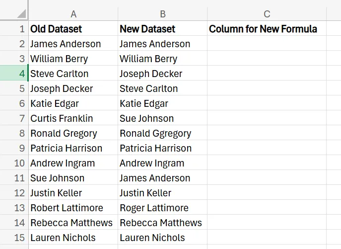
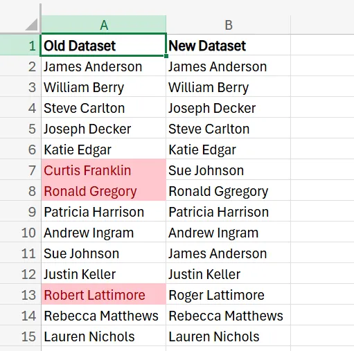
For the purposes of these examples, let’s say a company has created a new dataset for employee name data. The business wants to check if it matches up with the previous dataset, or if there are any issues they need to fix before deleting the older dataset and continuing on with the new one.

Using Formulas to Compare Columns

One way to compare two columns is by using formulas like IF, EXACT, or even VLOOKUP to see how the two columns stack up. Each of these begins with the same first step, which is to have your two datasets side by side in different columns. From there, you’ll create a third column next to them where you’ll eventually apply your formula.

IF

1. To use the IF formula, type =IF(A2=B2, "Match", "No Match") into the row in the third column next to the first set of names. If the names match, it’ll say “Match”, but if the names are different in any way, it’ll say “No Match”.

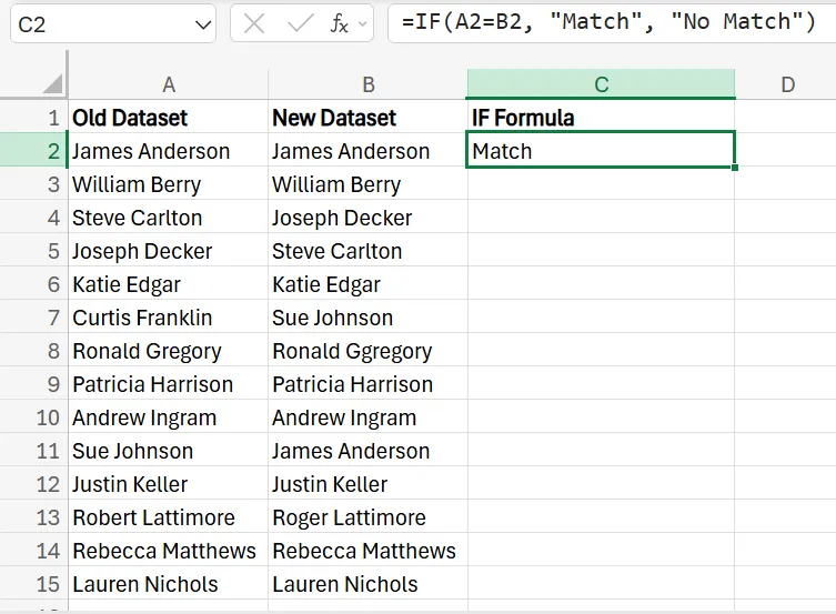
2. To drag the formula down across the rest of your dataset, just click the bottom right corner of the cell and drag it down until it covers all of the data.

EXACT

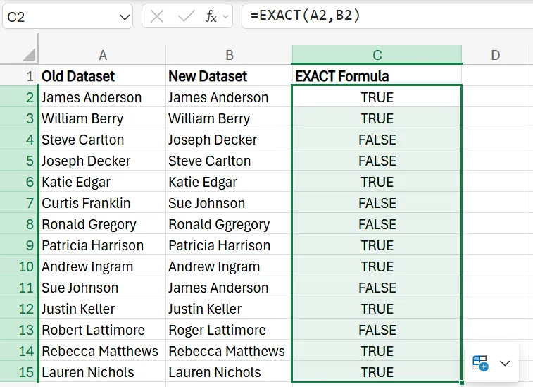
1. If you want to use the EXACT formula, locate the row in the third column right next to the first set of names and enter =EXACT (A2,B2). This essentially checks if a text string is the exact same as another, and provides either a “TRUE” or “FALSE’. Keep in mind that this method is case-sensitive.

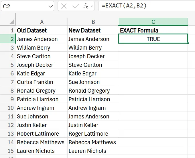
2. Once again, drag the formula down to apply it to the rest of the rows in the column.

VLOOKUP

While these two formulas help you check to ensure names are in the right order, if you just want to check if a name is in the column at all, you can use the VLOOKUP function and formula. This simply lets you check if certain values in one column are present in the other.

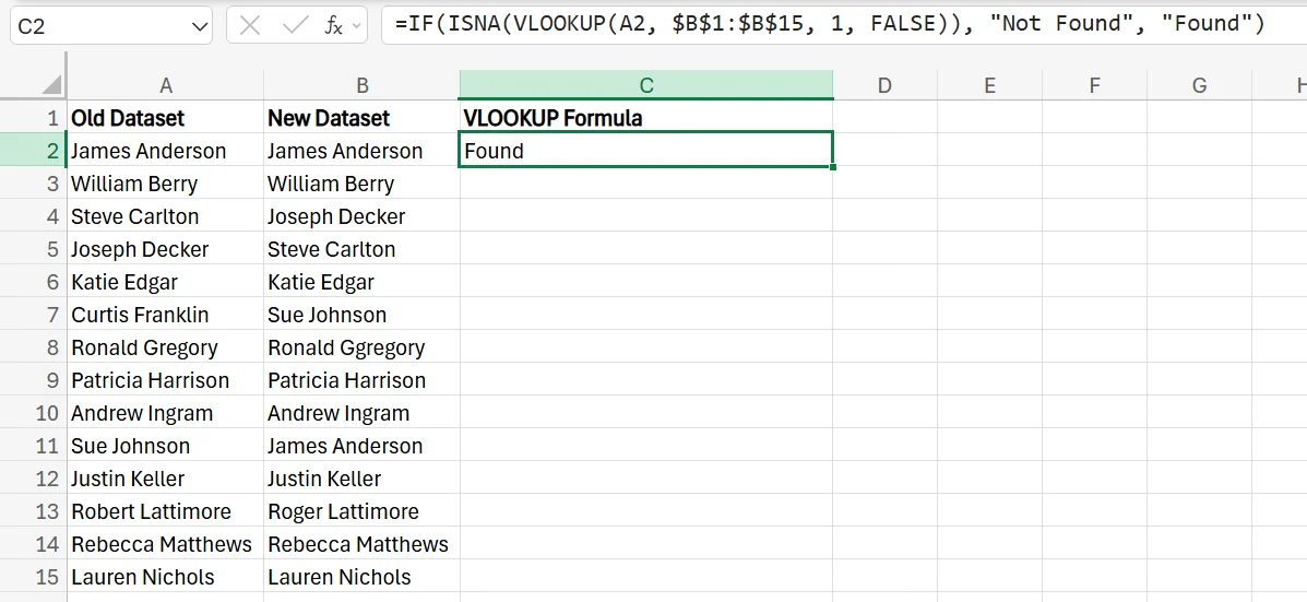
1. In the third column, type =IF(ISNA(VLOOKUP(A2, $B$1:$B$15, 1, FALSE)), "Not Found", "Found") in the cell next to the first set of names. This is essentially searching to see if the names in the first column are found anywhere in the second column. If they are, a “Found” appears, and if they’re not in the second column anywhere, a “Not Found” appears.

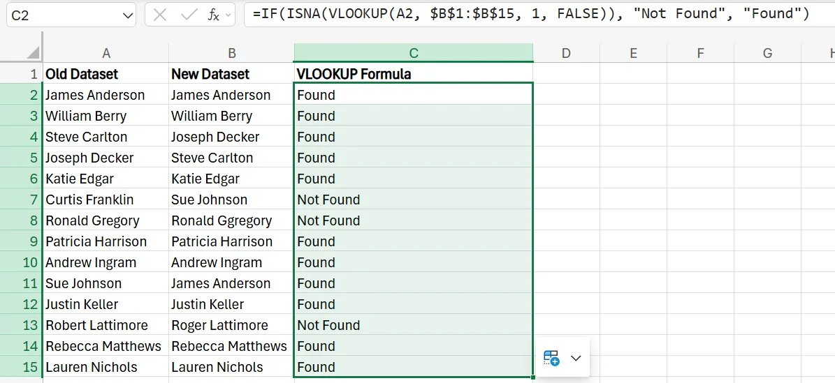
2. Drag the formula down, and make a note of any names that aren’t found in the second column so you can make the proper adjustments.

Utilising Conditional Formatting for Column Comparison

In addition to formulas, you may also use conditional formatting to compare columns. Let’s say, for this example, you want to highlight the names in the Old Dataset that don’t appear in the New Dataset.

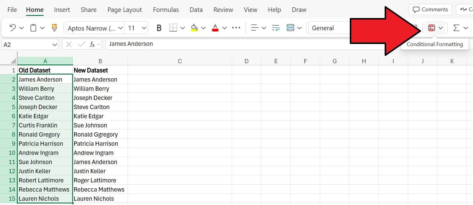
1. Begin by selecting the range of cells in the Old Dataset column. Once selected, go to the Home tab and press the Conditional Formatting button.

2. In the pop-up menu, click on New Rule.

3. In the Conditional Formatting menu, select the “Format cells where a formula is true” option.

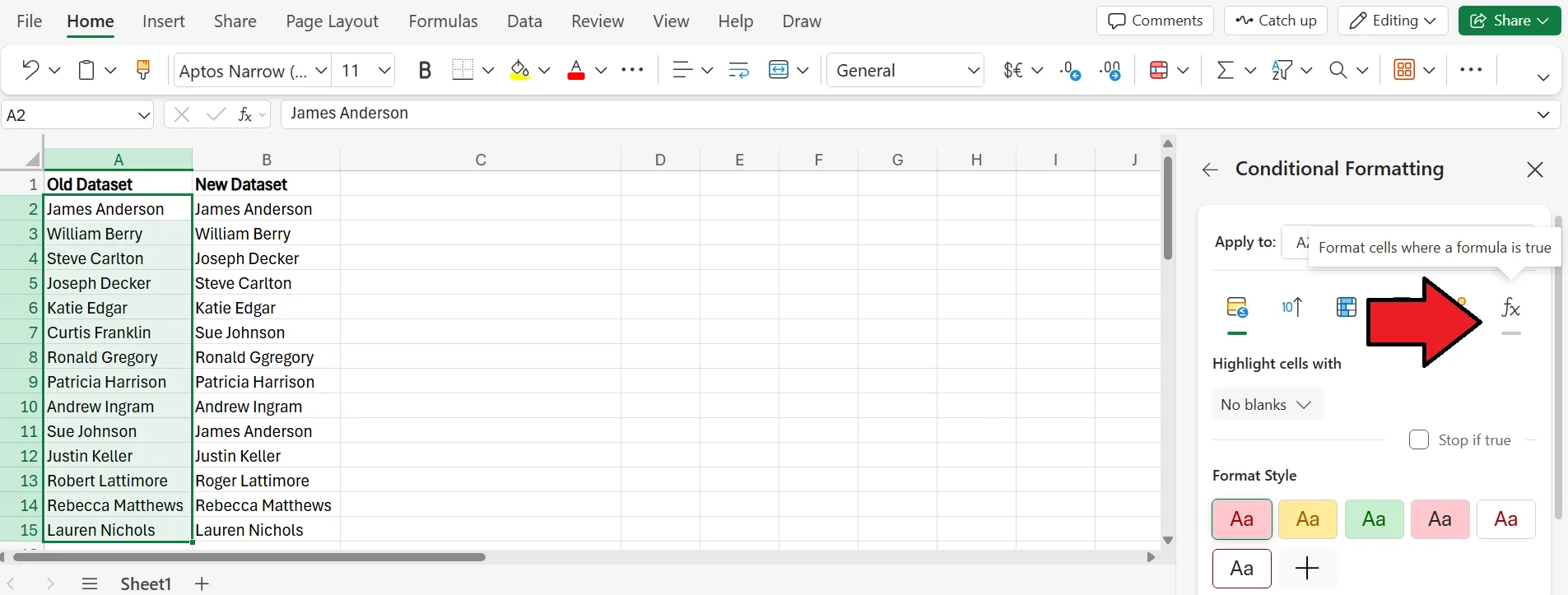
4. In the provided space, enter =ISERROR(MATCH(A2, $B$1:$B$15, 0)), choose the format style you prefer, and press Done. Once you do this, all of the names that appear in the old dataset, but not the new one, will be highlighted.

Best Practices for Data Comparison in Excel

Here are a couple of tips to keep in mind when comparing data in Excel to ensure it goes as smoothly as possible.

Ensure You’re Using Compatible Data

To ensure your comparison is accurate and not full of errors, make sure you’re using compatible types of data. For example, if you’re trying to compare numbers, and one column has actual numerical values and the other has the numbers written out, different functions and formulas will struggle to compare them. For best results, ensure both columns feature the same data, whether it be numbers or text/words.

Verify the Formulas

Many of the formulas you’re using to compare data in Excel are relatively long and include plenty of information. One simple bracket where it shouldn’t be, or using the wrong letter or number of a row/column, could throw off the entire calculation. As a result, always look over and verify that a formula is correct before applying it. Similarly, if you’re experiencing a strange error, one of the first things you should do is confirm that the formula is correct.

Label Everything

To ensure you don’t mix up one column for another, always ensure you label each one with a clear header so you know which dataset it represents. In a similar vein, make sure that your rows have the proper values in them, too.

Contact us today to learn more about how we can help you grow your business!