How to Implement Conditional Formatting in Excel Based on Another Cell

Conditional formatting in Excel is a useful tool that helps you format certain cells based on specific conditions or criteria that you’ve selected. This makes it easy and automatic to change the appearance and colour of different cells based on the values inside them. It’s great for identifying trends, patterns, outliers, and other important information quickly.

However, there may be times when you want to use conditional formatting based on the value in another cell. This guide goes over how to use Excel conditional formatting based on another cell​, why you may want to do it, and helps you troubleshoot common issues you may experience.

Our Excel instructor-led training courses cover a variety of topics suitable for both beginners and advanced users!

Understanding Conditional Formatting Based on Another Cell

This strategy involves referring to a cell to dictate how formatting is applied to a different cell, row, or column. It’s amazing to use in scenarios where the value in a certain cell has an impact on the appearance of an entire row or column.

For example, let’s say you have a benchmark number of sales that your sales team members need to meet every month. You can use conditional formatting so that the value in their sales column cell influences the overall appearance of their entire row in your spreadsheet.

If they’re selling above the benchmark, you could set conditions so that their entire row is highlighted green. And if they’re below the benchmark, you may have conditions that highlight it in red.

So now, when you add a new employee and drag the conditional formatting formula down, or adjust sales numbers for existing employees, you can automatically see how they’re performing vs. your expectations.

This specific conditional formatting technique is also great for highlighting projects past due based on due dates, monitoring inventory levels based on available stock, and a variety of other common business tasks.

Step-by-Step Guide to Setting Up Conditional Formatting Rules Based on Another Cell in Excel

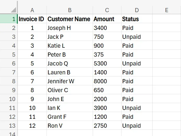
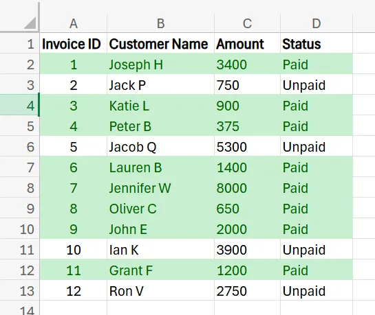
Let’s have a look at the steps involved in setting up conditional formatting rules based on another cell. While there are several different scenarios you may use this for, this example is going to focus on a company that wants to highlight all of its paid customer invoices in green in its spreadsheet to better be able to identify them quickly.

1. Begin by opening your spreadsheet that contains your invoices.

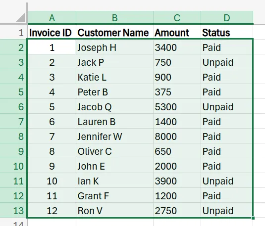
2. Select the entire range of cells that you’d like to apply the formatting to.

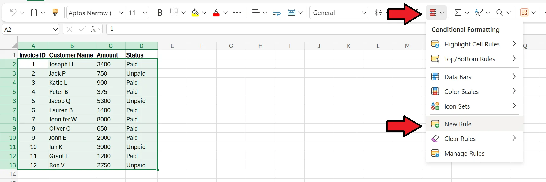
3. With the range selected, click on the Conditional Formatting button, and then select New Rule.

4. In the menu that pops up, choose the last option, which says “Format cells where a formula is true”.

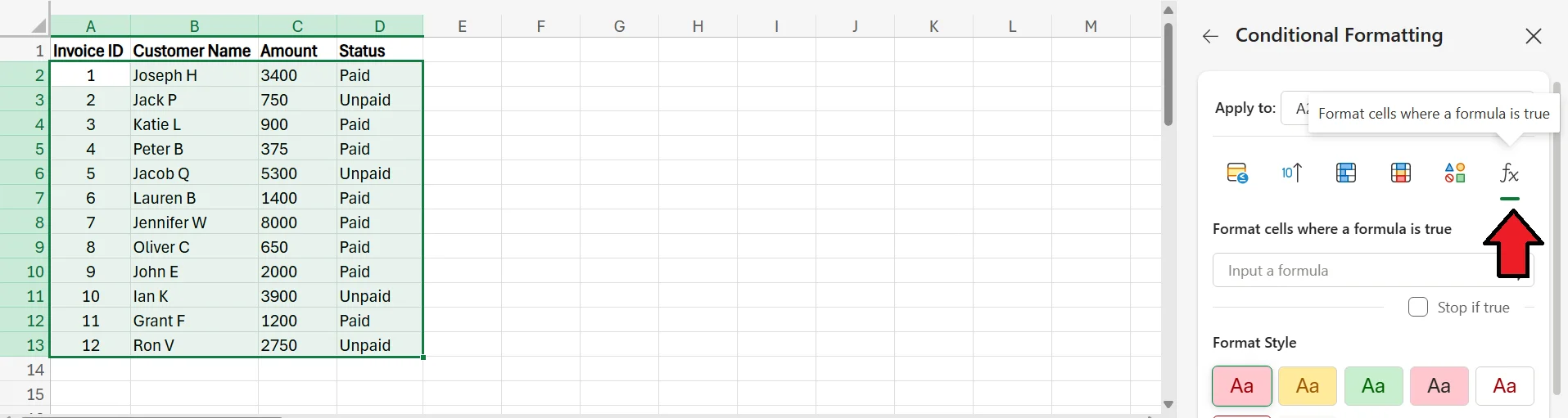
5. Enter the formula =$D2=”Paid” (if your “Status” cells are in a different column, use that letter instead of D). This formula is basically telling Excel to highlight a row if the cell in the “D” column for that row has the word “Paid” in it.

The dollar sign only being in front of the “D” in the formula ensures that the column is fixed, while the row is relative. While this won’t matter for now, if we eventually move the formula down and/or to the right, this dollar sign ensures the column reference stays the same, as we always want to be referencing the status of the invoices for this type of formatting.

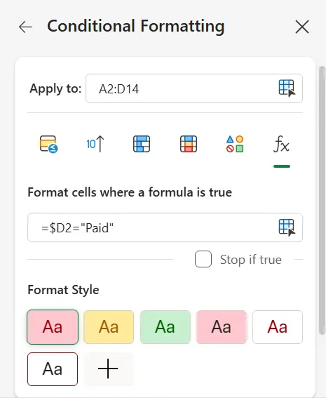
6. Next, choose the format style you prefer. You can choose one of the pre-made options, or design your own from scratch. Once you’re happy with the design, press Done and you’ll see the proper rows highlighted according to your format conditions and style.

Best Practices for Conditional Formatting Based on Another Cell

While it’s relatively straightforward to set up conditional formatting based on another cell, here are a few tips to ensure your calculations are correct and you don’t run into any issues.

Verify Your Formulas

One of the most common issues people run into while using this strategy is having incorrect formulas within their conditional formatting rules.

If you experience an error or are getting improper results, one of the first things to do is check and make sure that each formula contains the proper words, values, and references. If not, make adjustments until they’re correct and delivering the proper results.

It’s also a good idea to keep your formulas as simple as possible, so there’s less of a chance of making an error or not noticing a misspelling or a missing component within the formula.

Check the Range of Cells

Make sure to always check the range of cells you’ve selected before adding any conditional formatting. Even leaving out a single cell, row, or column may have major implications on how the formatting ends up looking.

Watch for Rule Conflicts

Excel lets you set up multiple conditional formatting rules for the same dataset, but these don’t always play nicely with one another. In fact, some rules may directly conflict with one another, leading to issues. If you experience any rule conflicts, you can address them by removing rules, adjusting rules, or altering rule priority.

In Excel, rules are applied in order, so the rules at the top of the list have priority over those on the bottom.

Get in touch today to learn more about how you can use Excel to grow your business!