How to Calculate Standard Error in Excel?

Excel helps you automatically perform a wide range of complex calculations to learn more about your data, with a much lower risk of manual error. One of these calculations is determining the standard error of your data.

This guide goes over how to calculate standard error in Excel, what it is, why it’s important, and more.

If you want to learn more about Excel’s different features, take a look at our instructor-led Excel training courses. They are suitable for both beginners and more experienced users.

What Is Standard Error?

The standard error is a measure that helps to show you how much the sample mean of a dataset may vary from the mean of the entire population. The smaller the standard error you arrive at, the more reliable your results are. Also, as you add more samples to your calculation, the size of your standard error shrinks.

Being able to calculate the standard error in Excel is important because it tells you how much you can trust the accuracy of a sample dataset. Companies may use standard error to help compare datasets, make decisions, ensure a sample properly represents a population, and closely evaluate datasets.

The Standard Error Formula Explained

The standard error formula in Excel is =STDEV.S(range)/SQRT(COUNT(range)). It’s essentially taking the standard deviation and dividing by the square root of the number of samples in the dataset.

Calculating Standard Error in Excel: A Step-by-Step Guide

Let’s go through a detailed example of how to calculate standard error in Excel. While there are several reasons a business may use a standard error calculation, for this example, let’s say a company wants to analyse its customer satisfaction ratings using the measure to see how accurately its sample reflects the entire customer base.

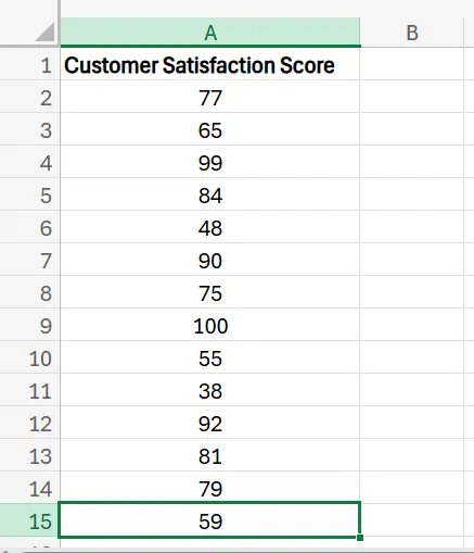
1. First, add your data to an Excel sheet and label it. In this case, we have a sample dataset of 14 customers and their customer satisfaction score, which is out of 100.

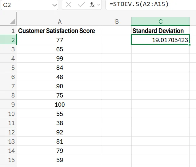
2. Find the standard deviation of the data, which is a measure of the variation of a dataset relative to its mean. To do this in Excel, simply choose a cell off to the side of your data, and enter =STDEV.S(range), with range being the cells you want to include in the calculation, which in this example are A2:A15.

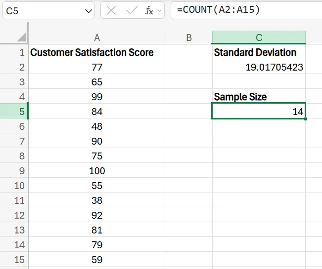
3. Once you’ve got the standard deviation, you need to find the sample size. With a small dataset, you may be able to manually count, but if you want a faster process (or if your dataset is too large to count quickly), use =COUNT(range). This will add up all of your samples and instantly display how many there are.

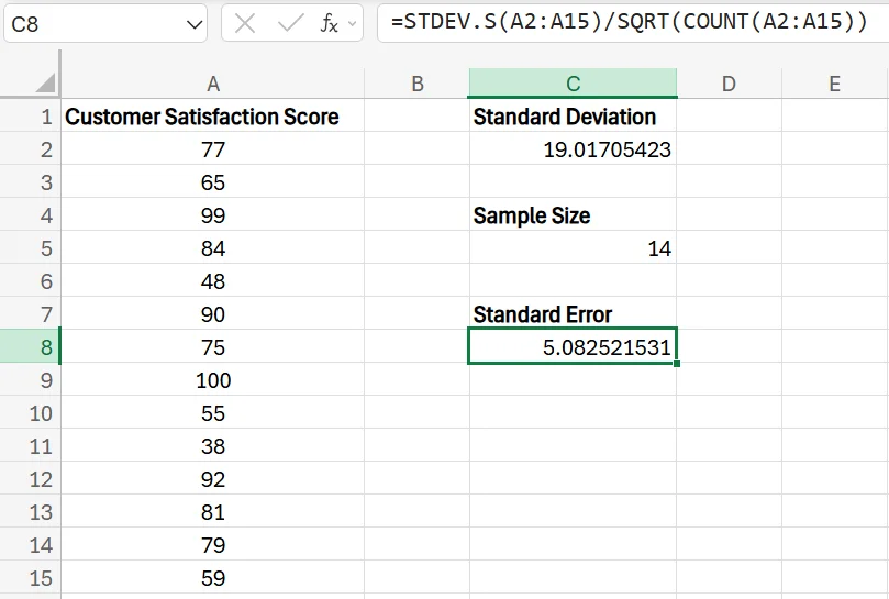
4. With both the standard deviation and the sample size, you’re ready to calculate the standard error. To do this, choose another cell and enter =STDEV.S(range)/SQRT(COUNT(range)). In this example, the formula will be =STDEV.S(A2:A15)/SQRT(COUNT(A2:A15)). After hitting Enter, your standard error is automatically calculated and displayed in the cell.

Optimising Your Standard Error Calculations

While calculating standard error in Excel only takes a few steps and is quite straightforward, there are some things you can do to ensure your results are as reliable and accurate as possible.

Increase Your Sample Size

Perhaps the best way to improve your standard error calculation is to increase your sample size. If possible, look to include as many samples in your dataset as possible. Sure, it may take more work to add additional samples into the sheet, but it’s well worth it to gain access to more reliable and precise data.

The closer you get to including your entire population in the calculation, the smaller your standard error will be, which signifies a more accurate dataset.

Use Random Sampling

Speaking of samples, it’s also crucial to ensure the samples you choose to include are random. If the samples you choose aren’t random, there’s a higher chance of bias occurring, which may skew results or lead to the sample not being an accurate representation of the population.

For example, let's say you want to evaluate customer satisfaction and need to decide which customers to include in the sample. Instead of just using your oldest customers, newest customers, or choosing based on name or job title, you need to choose them at random. This is much more likely to give you a sample that accurately reflects the characteristics of the entire population, and not just a subset or certain group.

Properly Label Everything

Another useful tip is to ensure that you properly label everything within the Excel spreadsheet. There’s a good chance you’ll have plenty of different numbers and types of data present there, and without the right labels, it's very easy to get confused about what number represents what.

If you accidentally mix up certain numbers, it may result in inaccurate calculations and errors that could take a lot of time and work to correct.

Contact us today to discuss how we can help your business grow by providing you with the tools and knowledge to succeed!