What is the Excel Formula for % Increase?

When comparing monthly or yearly sales in Excel, it’s often incredibly valuable to be able to quickly track the changes using percentages. However, doing these percentage calculations manually to see the difference is anything but fast.

Instead, why not use the Excel formula for percent increase? It helps you instantly see the percentage increase/difference between two numbers, without having to do the math by hand.

This guide is going to go through why you may use this formula, the steps needed to use it properly, and common mistakes to avoid to ensure you end up with accurate and proper results.

If you want to learn more about how your team can benefit from Excel, check out our instructor-led training courses!

What Is Percent Increase and Why Use It in Excel?

Percent increase is all about finding the difference between one value and another, and reflecting that difference in a percentage as opposed to simply using numbers. It helps you see just how much of a change there has been from one number to the next.

The Excel formula for percent increase is =(new value - old value)/old value.

There are several reasons your business may want to use this formula in Excel. As briefly mentioned in the intro, this formula is great for tracking sales growth over time. It can also help you judge employee sales performance over time, track your costs, view inventory changes, and even compare your monthly expenses.

In addition to these benefits, the formula also reduces the amount of manual work you’d need to do if you decided to calculate percentages by hand.

Step-by-Step Guide to Calculating Percent Increase in Excel

Now that you know more about the Excel formula for percent increase and what you can use it for, let’s go through the steps of using it properly. This example is going to focus on a company that wants to see the yearly percentage increase in sales over their last few years of business.

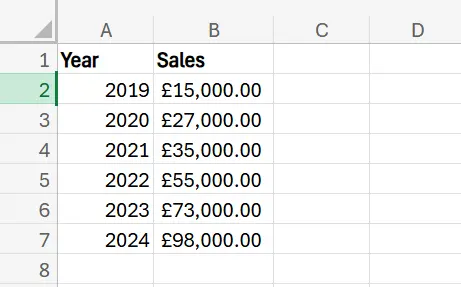
1. The first step is to set up your dataset properly. In this example, that means having a column for year, and then a column next to it that includes the sales for that year.

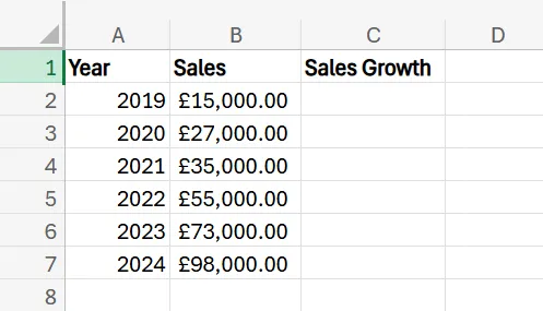
2. Next, add another column beside the Sales column that you can call Sales Growth. This is the column that’ll display the percentage increase in sales from one year to the next.

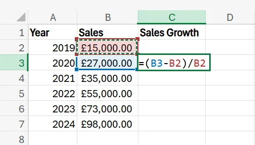
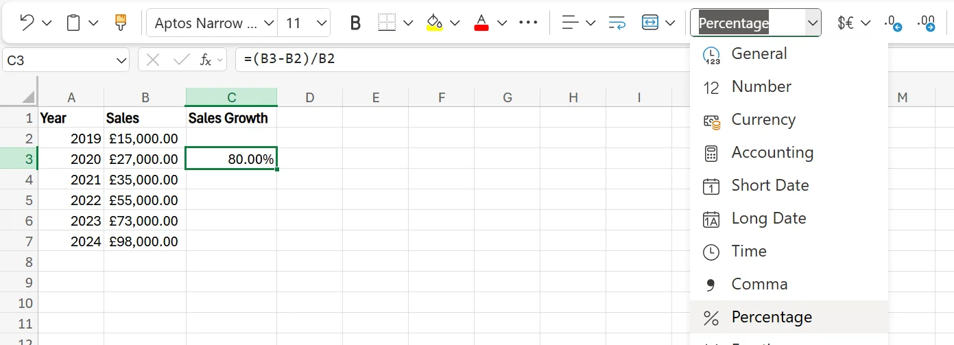
3. In the Sales Growth column in the cell next to 2020 (as we can’t judge the percentage increase in 2019 without data from 2018), enter the formula =(B3-B2)/B2. This is taking the 2020 sales, subtracting the 2019 sales, and then dividing that number by the 2019 sales.

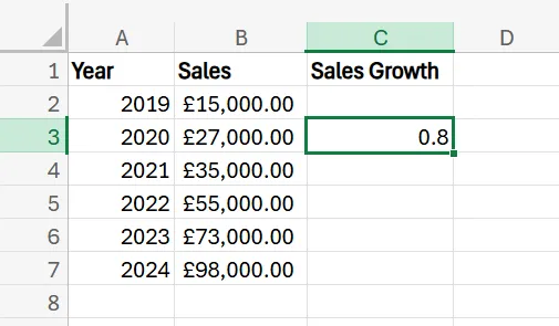
4. After confirming the formula by hitting enter, you’ll see a decimal answer.

5. To change this decimal to a percentage, simply click on the cell with the decimal in it, navigate to the Number Format section of the Excel ribbon, and select Percentage. The decimal should automatically turn into a percentage.

6. To carry over this formula to the rest of your yearly sales, simply click the bottom right corner of the cell with the percentage in it, and drag it down over the remaining cells in the column. You’ll now be able to see the percentage sales growth each year.

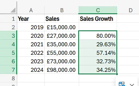
7. To confirm this worked properly, it can’t hurt to perform a few manual calculations to make sure everything adds up correctly.

Common Mistakes and How to Avoid Them

While using the Excel formula for percent increase properly is relatively easy and there are only a few steps involved, there are some mistakes you want to avoid.

Incorrectly Referencing Cells

One major issue you may run into is referencing incorrect cells within the formula. If you accidentally add a B4 in a place where a B3 should be, it could mess up the entire calculations in every other cell.

To avoid this issue, make sure to be careful when typing your formulas and always check them over to ensure every value is correct.

Similarly, watch out for other errors like missing certain operators, leaving out either the opening or closing bracket, or even using the wrong formula in general.

Not Formatting as a Percentage

Another mistake is forgetting to format your cells as a percentage. It’s a quick step that’s easy to miss, but goes a long way in helping the data look better and be easier to read and decipher. If you leave it as a decimal, it doesn’t stand out as much and doesn’t look as clean in your dataset, either.

Avoiding this issue is easy, as you just need to check to make sure you have the format for the cells set to Percentages as opposed to General, Numbers, or another option.

Contact us today to learn more about how we can help you and your team grow your business!