How to Use Pi in Excel

Pi is а constant in mathematics and represents the ratio of the circumference of a circle in relation to its diameter. It’s approximately equal to 3.14159, but in reality, it has an infinite number of decimal points, as it's an irrational number.

It’s incredibly important in math, as it helps calculate the areas of circles and cylinders, the volume of spheres, and assists in performing several other calculations in geometry and trigonometry. However, it has plenty of practical use cases for a wide variety of different businesses, as well.

This guide is going to take a closer look at pi, its practical use cases, and how to use it in Excel to support advanced data analytics.

Future Savvy’s Excel courses are designed to help you obtain practical skills that you can use in any business environment.

How to Use Pi in Excel

Instead of relying on manually entering the digits of pi when you want to use it, the PI function is a direct method to insert pi in Excel. There are several ways that you can make use of pi in Excel. Let’s have a look at a few of them, as well as go through step-by-step guides for each.

Displaying the Numerical Value of Pi

If you simply want to display the numerical value of Pi in a cell, all you need to do is choose your cell and enter the following syntax: =PI(). After you click Enter, the value of pi will appear in the cell.

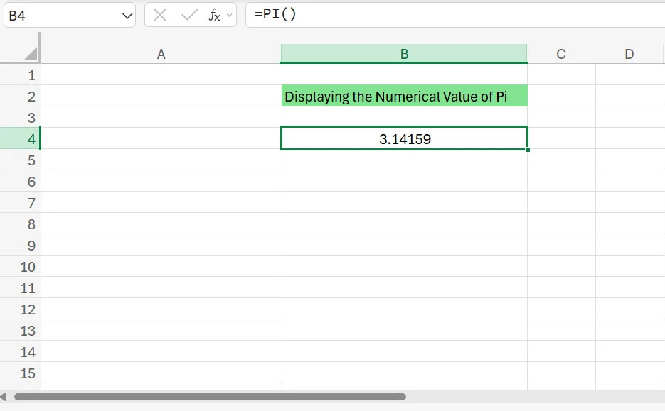
In total, Excel can calculate pi up to 14 decimal places.

Increasing Decimal Places for Pi

If you want to increase the decimal places for pi, all you need to do is click on the cell that contains pi, and then navigate to the Increase Decimal button and click it until you get to the number of decimal places you want.

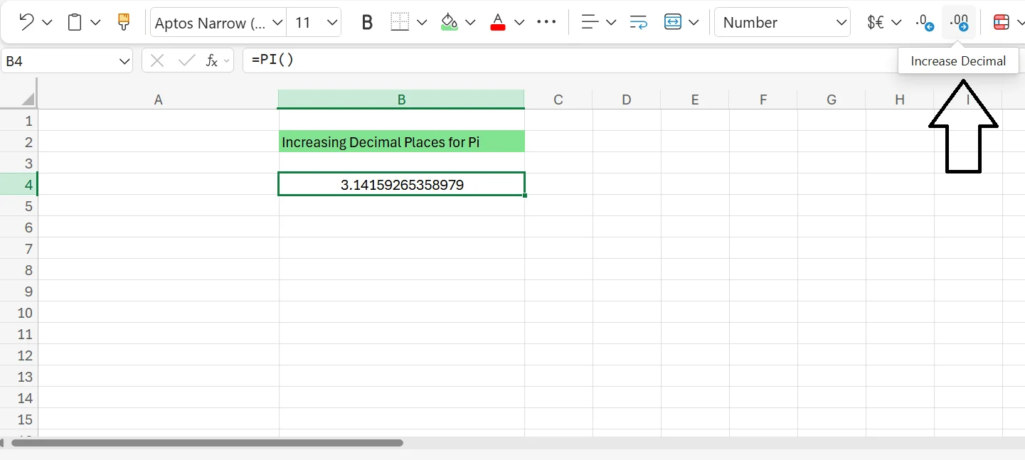
As mentioned in the previous section, Excel can only display pi up to 14 decimal places.

Inserting the Pi Symbol Into Excel

If you want to insert the pi symbol into Excel instead of the number it represents, you can do this in a couple of ways. First, you can simply go into the Symbols option in Excel, find Pi, and click the symbol to add it into a cell.

Another option is to use a keyboard shortcut to add it to a cell. The keyboard shortcut for pi is Alt + 227. By going to a cell and typing that shortcut, the symbol for pi should appear.

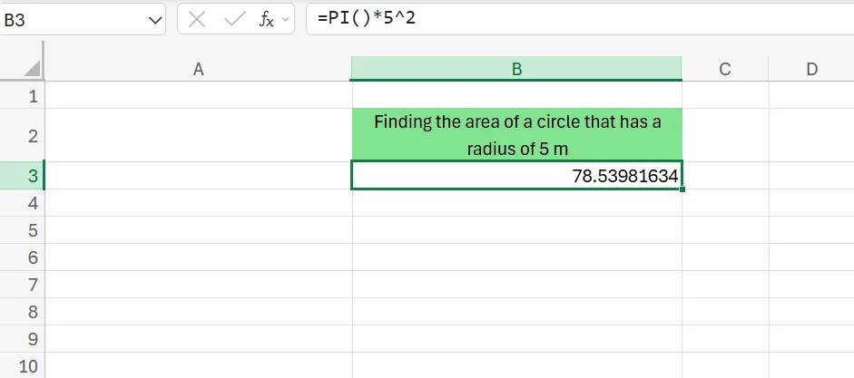
Embedding the Pi Function Into Mathematical Formulas

If you want to add the pi function to mathematical formulas, you need to simply begin with the syntax for pi and then add the rest of your calculation, whatever it may be.

For example, to find the area of a circle that has a radius of five metres, you’d use the following formula: =PI()*5^2. What this formula is doing is multiplying five by itself and then multiplying that number by pi to get the proper result, which in this case is just over 78.5 metres.

This is only one example of the many different ways you can use Pi in your mathematical formulas in Excel.

Potential Business Applications for Using Pi

There are several ways that using pi in Excel can help your business and your data analysis efforts. Firstly, using pi in Excel is great for performing complex circular or spherical calculations such as those used in financial modelling. Similarly, it also helps with engineering projects, prototyping, and building dashboards or digital signs.

For example, suppose you’re a company tasked with building a complex piece of architecture, like a bridge, tunnel, or arch. In that case, using pi in your calculations helps you determine proper load distribution, improve structural integrity, find the proper design/shape, and more.

But not only can pi help you ensure the project ends up being structurally sound, but it can also help you use mathematical calculations to determine how much material you’ll need to complete the project.

Pi can even help companies that design curved structures or circular products and aid in making fluid dynamics calculations to ensure proper flow rates. Of course, your business can also use it to directly integrate pi-based formulas into the business intelligence tools you use, such as Excel or Power BI.

If you want to learn more about Excel’s different functions and use them to grow your business, contact us today!